In this beginner-friendly guide to Laplacian Loss To, you’ll learn what the metric measures, how it’s computed, and when to use it to improve your models. The phrase Laplacian Loss To might sound technical at first, but its idea is straightforward: you pay attention to the smoothness and second-order structure of your predictions to reduce high-frequency noise and artifacts.
Laplacian Loss To: A Beginner’s Overview

Laplacian Loss To is a loss function that centers on the Laplacian operator, a mathematical tool that captures how a function curves on a grid. By targeting the Laplacian of predictions (or the residual error), this metric encourages outputs that are locally smooth while still allowing important edges to remain intact. In practice, Laplacian Loss To helps to regularize models beyond traditional pointwise errors, focusing on the structure of the prediction rather than just its absolute difference from the target.
What the term really means
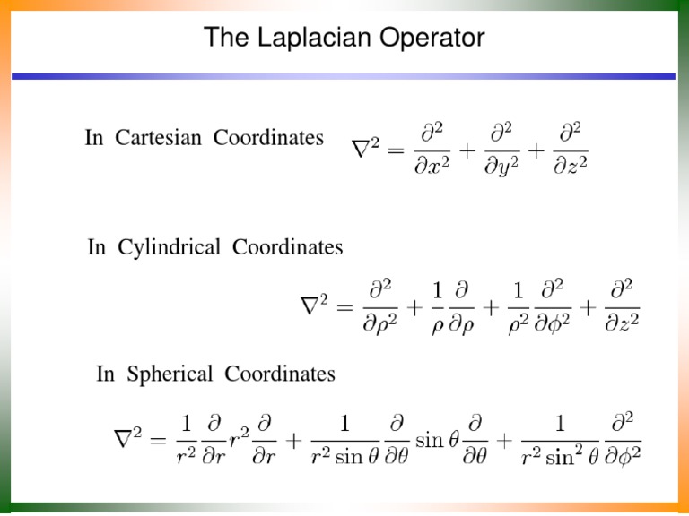
The Laplacian operator, denoted Δ, measures the divergence of the gradient. When applied to a gridlike signal or image, Δ highlights regions where the value changes rapidly in multiple directions. Using Laplacian Loss To means the optimization process minimizes how far the second-order variation deviates from zero, pushing the model toward outputs with coherent local patterns.
How Laplacian Loss To is defined and computed

There are a couple of common formulations of Laplacian Loss To. The exact choice depends on the data and the goal, but both share a focus on second-order structure rather than solely on absolute error.
Variant A: Laplacian of the prediction L = ||Δ ŷ||^2. This version promotes smooth outputs by penalizing strong curvature in the predicted signal or image.
Variant B: Laplacian of the residual L = ||Δ(y − ŷ)||^2. Here the emphasis is on making the error itself smooth, which can help reduce noisy high-frequency residuals without blurring important features.
In discrete, grid-based data, Δ is often implemented with a simple stencil, such as a 4-neighbor or 8-neighbor approximation. For a 2D image, a common discrete Laplacian kernel is applied to the prediction or the error, and the squared norm of the result is added to the training objective.
When to consider using Laplacian Loss To
Laplacian Loss To is particularly helpful when you want your model to learn coherent local structure, such as in image restoration, super-resolution, or any task where sharp edges should be preserved without amplifying noise. It complements pixelwise losses by focusing on second-order differences, which are often aligned with perceptual quality. If your data shows high-frequency artifacts after optimization, Laplacian Loss To can be a good ally in restoring natural-looking detail.
Practical tips for implementing Laplacian Loss To
To get the most from Laplacian Loss To, keep a few practical points in mind. The weighting of this loss relative to your primary objective matters a lot, as too much emphasis can blur fine details, while too little may not curb noise effectively. Start with a small coefficient and monitor both objective metrics and qualitative outputs. If your data lives on a boundary (edges of an image or signal), consider boundary handling carefully to avoid artificial artifacts. Finally, you can experiment with either Laplacian of prediction or Laplacian of residual, depending on whether your priority is smoothness of the output or cleanliness of the error signal.
Key Points
- Encourages local smoothness while preserving meaningful edges in grid-like data.
- Two common forms: Laplacian of the prediction or Laplacian of the residual; choose based on your goal.
- Discrete implementation uses a Laplacian stencil; the exact kernel affects sensitivity to boundaries.
- Best used as a regularizer with a carefully tuned weight alongside standard losses.
- Helpful for image-related tasks and any domain where second-order structure matters.
Common use cases and best practices

In image processing tasks such as denoising, inpainting, or super-resolution, Laplacian Loss To often improves perceptual quality by reducing patchy noise that standard losses miss. For time-series or 1D signals, applying a Laplacian-like second-derivative penalty can help suppress abrupt oscillations without blurring the overall trend. When combining Laplacian Loss To with other losses, consider scheduling or adaptive weighting to maintain a balance between fidelity and smoothness. Regularly visualize outputs during training to catch any unintended smoothing of important features early.
Bottom line on use cases
If your model struggles with crisp edges or noise amplification, Laplacian Loss To is worth a try. It adds a structural lens to optimization, pushing predictions toward plausible local behavior while preserving essential patterns in the data.
What is the Laplacian operator, and why does it matter for this loss?
+The Laplacian Δ captures how a function curves by summing its second derivatives. In a grid, applying Δ highlights rapid changes in multiple directions. Using Laplacian Loss To leverages these curvature cues to encourage smooth, coherent predictions and limit noisy high-frequency artifacts.
How does Laplacian Loss To differ from standard MSE loss?
+Mean Squared Error (MSE) focuses on pointwise differences between prediction and target. Laplacian Loss To, by contrast, emphasizes second-order structure, penalizing sharp curvature or noisy residuals. This can improve perceptual quality and reduce artifacts that MSE alone may miss.
What should I watch out for when weighting Laplacian Loss To?
+Setting the weight too high can overly smooth results and erase important details; too low, and the loss may not exert noticeable influence. A common approach is to start with a small coefficient, monitor qualitative outputs, and adjust based on validation metrics and visual inspection.
Can Laplacian Loss To be used outside images, like in 1D signals or graphs?
+Yes. For 1D signals, a 1D discrete Laplacian stencil applies. For graph-structured data, you can adapt the Laplacian to the graph Laplacian operator. The core idea remains: penalize second-order variation to encourage smoother, structurally coherent outputs.
Is Laplacian Loss To compatible with other losses in a multi-task setup?
+Absolutely. In multi-task learning, Laplacian Loss To can be added as an auxiliary loss to guide shared representations toward smoother, more consistent outputs across tasks. Tuning the relative weight per task helps maintain balanced learning.